Stockpile volume computation with Open3D
First of all, you’ll need a Point Cloud of the stockpile. I’m going to use a .ply of an IntelRealSense-captured small stockpile. However, any other imaging technique resulting in a Point Cloud would be equally valid.

Check the code at my Github.
1. Orienting the Point Cloud
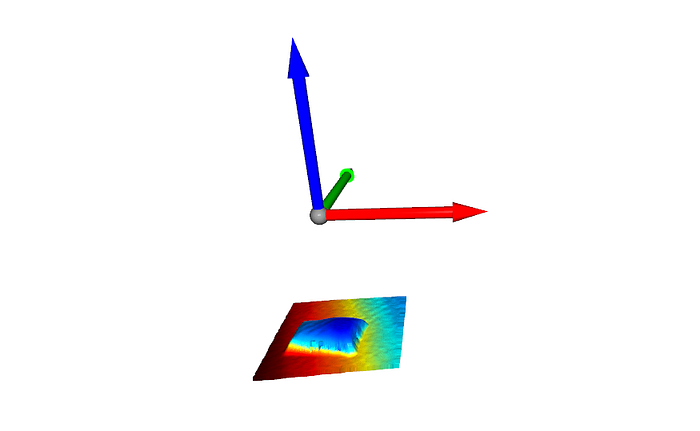
Let’s open our Point Cloud and check where in the cartesian 3D space it is located. Open3D has out-of-the-box tools for Point Cloud visualization. We will also add axes to our visualization so that we can locate the stockpile:
pcd = o3d.io.read_point_cloud("data/stockpile.ply")
axes = o3d.geometry.TriangleMesh.create_coordinate_frame()
o3d.visualization.draw_geometries([pcd, axes])
We can see our stockpile and the floor. We can also see that it is unoriented with respect to the axes. In order to compute the volume, we need to make the floor parallel to the XY plane and to translate it to the origin. To do so we need to segment the floor. Lucky again, Open3D has us covered:
plane_model, inliers = pcd.segment_plane(distance_threshold=0.01,
                                         ransac_n=3,
                                         num_iterations=10000)[a, b, c, d] = plane_model
plane_pcd = pcd.select_by_index(inliers)
plane_pcd.paint_uniform_color([1.0, 0, 0])
stockpile_pcd = pcd.select_by_index(inliers, invert=True)
stockpile_pcd.paint_uniform_color([0, 0, 1.0])o3d.visualization.draw_geometries([plane_pcd, stockpile_pcd, axes])

Now that we have segmented the floor plane, we can use a few mathemagics to bring the floor to the XY plane by rotating and translating the Point Cloud:
plane_pcd = plane_pcd.translate((0,0,d/c))
stockpile_pcd = stockpile_pcd.translate((0,0,d/c))cos_theta = c / math.sqrt(a**2 + b**2 + c**2)
sin_theta = math.sqrt((a**2+b**2)/(a**2 + b**2 + c**2))
u_1 = b / math.sqrt(a**2 + b**2 )
u_2 = -a / math.sqrt(a**2 + b**2)rotation_matrix = np.array([[cos_theta + u_1**2 * (1-cos_theta), u_1*u_2*(1-cos_theta), u_2*sin_theta],
                            [u_1*u_2*(1-cos_theta), cos_theta + u_2**2*(1- cos_theta), -u_1*sin_theta],
                            [-u_2*sin_theta, u_1*sin_theta, cos_theta]])plane_pcd.rotate(rotation_matrix)
stockpile_pcd.rotate(rotation_matrix)
o3d.visualization.draw_geometries([plane_pcd, stockpile_pcd, axes])

We can discard the floor, as we are only concerned about the stockpile.
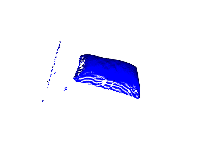
o3d.visualization.draw_geometries([stockpile_pcd])
As we can see, we have some wrongly segmented points, especially in the border of the 3D image. We will need to remove these outliers. You know where this is going, Open3D has a function just for this:
cl, ind = stockpile_pcd.remove_statistical_outlier(nb_neighbors=30,
                                                    std_ratio=2.0)
stockpile_pcd = stockpile_pcd.select_by_index(ind)
o3d.visualization.draw_geometries([stockpile_pcd])
Okay, we finally have our stockpile Point Cloud segmented, and correctly oriented. We can now jump to the volume computation part. Yay!
2. Computing the volume
We can not compute the volume from a Point Cloud, we need a mesh. To get from Point Cloud to a mesh we can use surface reconstruction algorithms. Surface reconstruction is an ill-posed problem, meaning there is no perfect solution and algorithms are based on heuristics. However, we can avoid these algorithms by exploiting one special characteristic of a stockpile (or any terrain really), which is that the surface is bound by the XY plane. No 2 points will have the same x and y, and looking to the surface from above to the XY plane we will see a “plain ”surface, which is to say that if at any point we cross the XY plane perpendicularly, we will only cross our surface once.
We will build the triangularization for the surface reconstruction in the 2D space. We will project out PCD to the XY plane by removing the Z value. We will get the triangulation of our 2D points with the Delaunay algorithm. Then we will keep the triangles outputted by Delaunay but we will use the 3D vertices instead of the 2D ones. This approach is sometimes called “Delaunay 2.5D”
This may sound convoluted, but it is easy to see in the code:
downpdc = stockpile_pcd.voxel_down_sample(voxel_size=0.05)
xyz = np.asarray(downpdc.points)
xy_catalog = []
for point in xyz:
    xy_catalog.append([point[0], point[1]])
tri = Delaunay(np.array(xy_catalog)
tri will give us the indexes of the triangles. In the 2D space this looks like:

Using the triangles with the 3D points will give us the surface of our stockpile:
surface = o3d.geometry.TriangleMesh()
surface.vertices = o3d.utility.Vector3dVector(xyz)
surface.triangles = o3d.utility.Vector3iVector(tri.simplices)
o3d.visualization.draw_geometries([surface], mesh_show_wireframe=True)
Once we have the surface, we are ready to get the volume. Different approaches can be followed. I will compute the volume of each triangle of the surface to the XY plane (height 0). Then just add the volumes of all the triangles.
Triangles in Open3D meshes define the indexes of the vertices, not the vertices, so we need to translate the triangles so that their values are actually 3D points and not indices to the vertices list:
def get_triangles_vertices(triangles, vertices):
    triangles_vertices = []
    for triangle in triangles:
        new_triangles_vertices = [vertices[triangle[0]], vertices[triangle[1]], vertices[triangle[2]]]
        triangles_vertices.append(new_triangles_vertices)
    return np.array(triangles_vertices)
Then we will need a function to compute the volume under each triangle. Following the article of the Bourbakian mathematician Kevin Brown, we can define such function as:
def volume_under_triangle(triangle):
    p1, p2, p3 = triangle
    x1, y1, z1 = p1
    x2, y2, z2 = p2
    x3, y3, z3 = p3
    return abs((z1+z2+z3)*(x1*y2-x2*y1+x2*y3-x3*y2+x3*y1-x1*y3)/6)
Then, getting the volume of our stockpile is as easy as adding the volumes of all the triangles:
volume = reduce(lambda a, b: a + volume_under_triangle(b), get_triangles_vertices(surface.triangles, surface.vertices), 0)print(f"The volume of the stockpile is: {round(volume, 4)} m3")
I hope that you enjoyed this article 😃. Feel free to contact me if any point is not clear enough!
